Understanding Population Variance and Sample Variance Formulas
Understanding Population Variance and Sample Variance Formulas
In my data science learning journey, I set a goal to really understand the fundamental topics before moving on to advanced ones. Instead of striving to learn as many things as I can, I slow down and really understand how things work under the hood. This weekend, I revisited my statistics basics and thought of writing about an easy way to understand variance.
In this article, I will discuss:
- How to make sense of variance by using visuals
- Why variance calculation uses squares
- Why population variance and sample variance have different denominators
- Writing a variance function from scratch
First, let do a little refresher on what variance is:
Variance is a statistical measure that explains how far away data points are from the mean, and hence from each other.
- A variance of zero means all data is similar (we have only one data point)
- The higher the variance, the more disperse our data is (the data points are far away from the mean and from each other)
- The lower the variance, the less disperse the data is (data points close to the mean and to each other)
- Variance cannot be negative!
How to make sense of variance by using visuals
The variance is calculated as
\[\begin{align} \text{Var}(X) &= \frac{1}{n}\left((x_1-\mu)^2+(x_2-\mu)^2+\ldots+(x_n-\mu)^2\right) \\ &= \frac{1}{N}\sum_{i=1}^n (x_i-\mu)^2 \end{align}\]Where,
- \(x_{i}\) is the ith value in the data set;
- \(\mu\) is the population mean;
- \(N\) is the number of values.
In other words, the variance is the average of the squared deviations from the mean.
Let’s use python’s scikit-learn built-in dataset, the Iris dataset, to break down this formula. Please find the full notebook on my github
We will import all necessary libraries first:
# Import libraries
import numpy as np
import pandas as pd
import matplotlib.pyplot as plt
import seaborn as sns
from sklearn.datasets import load_iris
Loading and visualizing the first 7 rows of the data
# Load the dataset
iris = load_iris()
df = pd.DataFrame(iris.data, columns = iris.feature_names)
df.head()
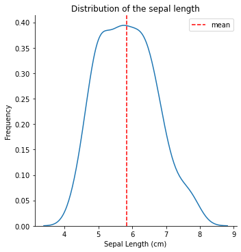
For simplicity we will exclusively use the first column of the data, but the process is the same! By visualizing the distribution of sepal length, we see that is pretty much normally distributed with a mean of around 5.8 cm.
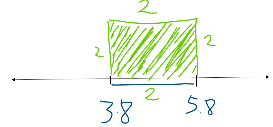
The first step to calculate variance is finding the distance between each data point and the mean. Consider a flower of a 3.8cm sepal length. This data point is two centimetres away from the mean (5.8 cm). If we square the difference, we get 4, which is the area of the square of sides of 2.
We do the same for every other data point in our dataset to form different squares. The variance is the mean of the area of those squares together. The figure below shows the distribution of the squared differences along with the distribution of sepal lengths. Note that I immediately calculated and plotted the mean of the squared differences, which is the Variance.
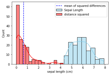
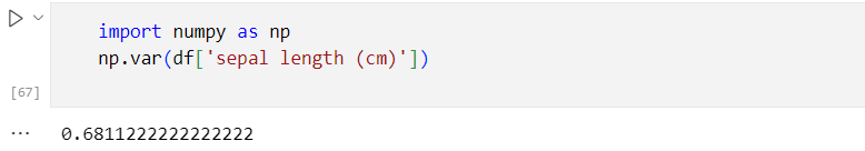
In this case, the variance is close to 0.7, which is the same as the one calculated using numpy.
Why variance calculation uses squares
Why do we square the difference and not take absolute values? This, alone, can be a post in itself explaining advantages and disadvantages of squaring the differences. However, in short, squaring the differences in the variance serves two main purposes:
- It penalizes the outliers (larger dispersions from the mean) more than the data points closer to the mean, and
- It ensures were are not summing negative values — this prevents the distances above the mean from cancelling out with those below, which would result in a variance of zero
If you want to read more about this, please refer to this StackExchange post!
Why population variance and sample variance have different denominators
The variance we calculated above is referred to population variance. However, in practice, we rarely use population variance since we are working with samples taken from the study population. When dealing with a sample, we calculate sample variance instead.
Our goal is for the variation in our sample (sample variance) to estimate the variation in the population as accurately as possible. Since the population mean is unknown, we estimate it using the sample mean. In this process we are already introducing bias in our variance, so we need to correct for that bias by multiplying the population variance with n/(n-1), where n is the number of observations. This bias correction is known as Bessel’s correction. If we didn’t correct for this bias, the variance obtained would be a biased estimator of the population variance
After correcting for the bias, the formula becomes:
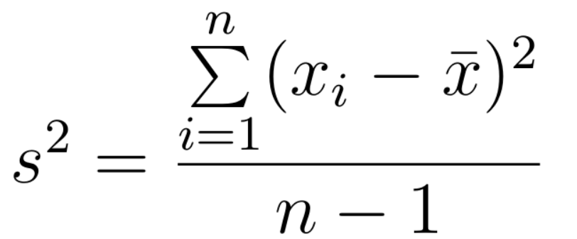
where, x_i is the ith value in the data set; x̄ is the sample mean; n is the number of observations;
Note that the formula is the almost the same as that of population variance except that we take n minus one degree of freedom as the denominator for the sample variance.
Now to the best part….Let’s write our own variance function from scatch :
def var_calc(x):
    """
    Calculate population variance of a dataset.

    Parameters
    ----------
    x : array-like
        The dataset whose variance is to be calculated.

    Returns
    -------
    float
        The variance of the dataset.
    """
    n = len(x)      # number of data points
    mean = sum(x)/n # mean of the data
    diff_sq = [(x_i - mean)**2 for x_i in x] # squared difference from the mean
    return sum(diff_sq)/(n) # population variance
Testing it out…
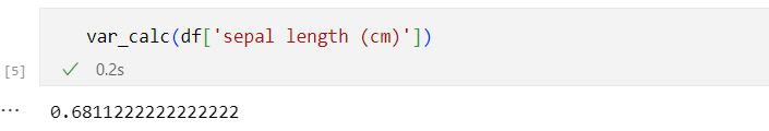
There you have it!! Now we know what variance is, why we square deviations from the mean, and the difference between population and sample variance. Above all, if we wanted, we wouldn’t have to rely on numpy’s variance function to calculate our own variance. Isn’t that amazing? I think it is!!!
À bientôt!!